Vector Indexes: HNSW vs IVFFLAT vs IVF_RaBitQ

The topic of vector indexing has been around ever since we store vectors in databases at large scale. Their purpose is to find the closest vectors to our query vector in a faster manner, using some pre-made structures, which eliminate doing the whole computation at query time. We all want fast and accurate queries, but at what cost? Are there any pitfalls? In this article we try to give answer to these questions.

Achieving good recall at high speed is a balancing act. We might need to sacrifice some recall in exchange for some speed and vice-versa. Vector indices are not omnipotent magic crystal balls. They are a kind of magic crystal ball that have a confined way of correct usage. 

In this article, we have compared three types of vector indexes. If we take a look around the different vector database implementations, we will see that most of the times HNSW is the default or is available as a vector index option, basically being the gold standard index to use. Other popular approaches are generally IVF based, among which the original IVFFLAT is the most common. That’s why we choose the following 3 to compare: HNSW, IVFFLAT and IVF_RaBitQ.  We have dived into the most important questions regarding the mentioned vector index types. 

Hierarchical Navigable Small World - HNSW

Let’s start with the most well-known and probably the most used out of all - HNSW. Generally speaking this index type is the most widespread, thanks to it’s very fast query times, while retaining high recall in most cases. In some other cases, where the table is constantly changing, it still can work very well, but it definitely needs some caution.

HNSW index does the distance pre-computation in the form of building an Approximate Nearest Neighbour -- ANN --

graph. The top layers contain representative nodes and the bottom layer contains the full data connections. The graph has an increasing density towards the bottom layers, which is achieved by assigning the nodes with an exponentially decaying distribution, from layer 0 (bottom) to layer L (top).

When building the index, for each vector perform a best-first search of width ef_construction around the current insertion point to gather a set of candidate neighbours. From those candidates, select up to M closest points from all layers. These parameters make or brake this index type, but they are also very hard to correctly specify.

Our query vector enters at the most sparse layer, so there are drastically less comparisons to make to get the initial “direction“. As we progress downwards in the graph, we hope to get closer and closer to our wanted records, the approximate nearest neighbours.

To find the closest nodes to a query, HNSW starts at the top layer with an entry point and performs a greedy search. It then descends layer by layer, refining the search at each level until reaching the bottom layer, where the final approximate nearest neighbours are found.

This hierarchical graph structure enables very fast search – the search complexity is essentially sub-linear (often near-logarithmic in N) for large high-dimensional datasets, because the upper layers quickly narrow down the search region and the graph’s small-world nature ensures few hops are needed to reach close neighbours.

Now we will touch on the questions which are crucial to answer, in order to use the index properly.

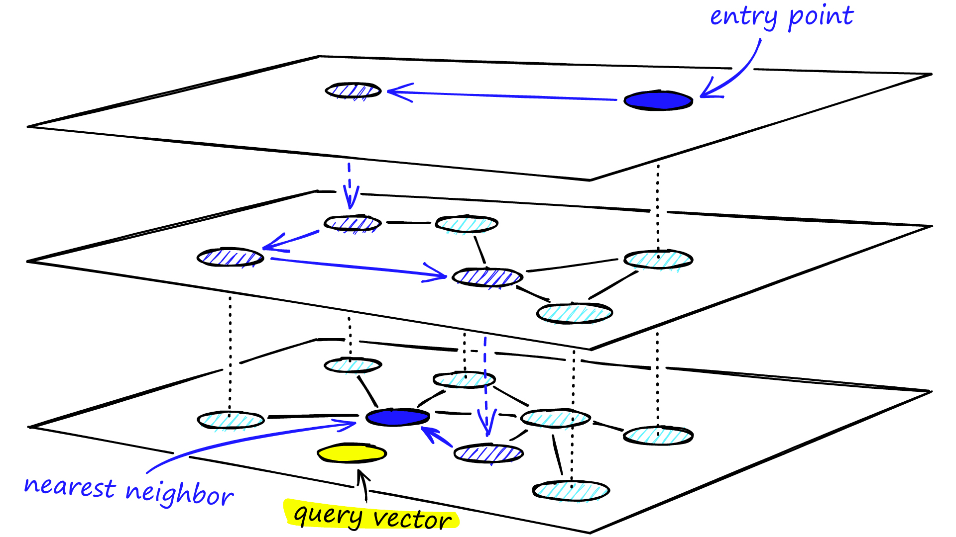
Image from: Hierarchical Navigable Small Worlds (HNSW) 

Parameters

What happens when a new record enters the table?

• The algorithm first samples a “max layer” for the new vector via geometric distribution, essentially as a node in build time.
• Starting from the top layer of the existing graph, it performs a greedy search to find the closest entry point at that layer, then “drops” down layer by layer until it reaches the sampled insertion layer.
• At each layer, it identifies the M nearest neighbours and connects the new node to them, pruning any neighbour lists that exceed the maximum size to keep the graph sparse.

The good news is that new entries slot right in, the bad news is that if M is not sufficient, you can actually create unreachable nodes, due to pruning.

What happens when a record is deleted from the table?

The way the given implementation handles deletion is one of the most important things for an HNSW index to work well. If you delete a node which is present not just at the bottom layer, you are deleting a potential entry point for future queries, and all of the deleted node’s connections. Such nodes usually referred to as tombstones. Now, if you have a table which is basically almost static, the way an implementation handles these tombstones might be completely irrelevant to you. But if you have a very lively one, this is crucial.

Some implementations remove tombstones immediately. This in itself can make some nodes less, or totally unreachable, since we are deleting a node with all of it’s edges. Every deletion makes the original index graph less and less connected, which can cause degradation, despite constant updates. Other implementations leave them in for an extend period of time, and after their amount exceeds a threshold, a delayed cleanup or “vacuum” procedure kicks in which refreshes the index, as well as deletes the tombstones.

In our experience, the better option is to leave the tombstones in, and reindexing frequently. A great HNSW implementation is done by qdrant, more on that here: Indexing - Qdrant 

What happens when you filter the indexed table?

Default behaviour is to preform the search using the index first, filtering comes second. Systems supporting pre-filtering can avoid these pitfalls by narrowing the search space up-front, but that can worsen the correctness of the index. The main issue with this approach remains that the index was built on the premise of the whole table considered as potential search results. If the records mix well enough from category to category, it might just be the case that the closest neighbours of a search candidate are meaningless or there is not enough of them after the filtering.

A solution could be indexing on tables partially. This works best if you store more than one type of data in one table and you only need one type at a time. That way you can partially index the pre-filtered table, and search via index on that.
11.8. Partial Indexes 

How to know when to reindex

There are no exact recommended metrics to decide this, the Vacuum process is automatic at 20%, but there is no general no rule of thumb. One thing you might be able to do, is that if you have a table specific benchmark, the drop of recall can be a good indicator, if you have such benchmark. If not, others usually use the drop of returned results as an indicator, but that might be a bit too late.

To summarise, HNSW is a very reliable index type with generally the fastest query times. But depending on our use case, it is wise to take some caution when choosing an implementation and parametrising the index.

Pros:

• Most widespread index type, available in almost all vector databases.
• It is generally considered to be the one of the fastest indexes in terms of query speed.
• Scales well with high-dimensional vectors.

Cons:

• Slow index build time, with certain applications frequent rebuilding might be necessary.
• Handling of deleted records depends on the implementation → It is crucial to use a good implementation like Qdrant.

Inverted File Flat - IVFFLAT

IVFFLAT is a clustering-based vector index that speeds up search by limiting comparisons to a subset of the dataset. In an offline training phase, the algorithm uses k-means clustering, partition vectors into clusters often referred as nlist. Mathematically speaking these clusters are Voronoi cells. Each cell has a centroid, and an inverted list of member vectors. A quick refresher about K-means:

Steps:

• Initialize: Choose K random points as initial cluster centroids.
• Assign: Assign each data point to the nearest centroid (using some distance, usually Euclidean).
• Update: Compute new centroids as the average of all points assigned to each cluster.
• Repeat: Iterate steps 2–3 until assignments stop changing / maximum number of iterations is reached.

You can swap out the regular algorithm to Spherical K-means, which is often recommended for text embeddings:

Steps:

• Normalise all input vectors to unit length (i.e., project them onto the unit hypersphere).
• Initialise K unit-length centroids.
• Assign each point to the nearest centroid based on cosine similarity.
• Update centroids by computing the mean of assigned vectors, then re-normalise to unit length.
• Repeat until convergence.

The index stores these lists and the centroids. Querying is done in two stages: 

• The query vector is compared to all centroids to find the closest clusters (the top nprobe amount of clusters are selected). 
• The search then examines only those few clusters, scanning through their member vectors to find the nearest neighbours to the query. 

Image from: Voronoi diagram

By avoiding brute-force over all vectors and only searching a small fraction of clusters, IVF achieves much lower query time than a flat linear scan. The “Flat” in IVFFLAT means that vectors are stored in full precision in the lists. This preserves accuracy, but the search remains approximate since we don’t scan every cluster – if the true nearest neighbour falls in a cluster outside the probed ones, it may be missed. In essence, IVFFLAT is a coarse quantisation approach, limiting the number of vectors checked, rather than the “resolution“ of them.

Paramaters

What happens when a new record enters the table?

It finds the nearest already existing centroid, and appends the new entry it to it’s list. Since new entries are classified one by one to an existing cell, if you insert members of an imaginary “new cluster“ one by one, they will not create their own cluster, but rather will be inserted to an existing ones. To avoid this behaviour, after a given amount of new entries, rebuilding the index is advised, similarly to HNSW.

What happens when a record is deleted from the table?

In IVFFLAT this has a way less severe impact, since a record is just a member of a list, which only affects the “True” centroid. Since the deleted member was used to calculate the centroid, the mean of the remaining list members (true centroid) and the calculated centroid will differ from each other. More importantly, deletion of a member doesn’t affect other connections, since in the case of IVFFLAT, there is no “unreachable node”. This is a big upside against HNSW.

What happens when you filter the indexed table?

The same could be repeated here, as with HNSW. Filtering here is also done post search, but partial indexing for example in Postgres is also available for this index type.

How to know when to reindex

Again, there is no exact rule to decide this. A rule of thumb could be that if N is the number of vectors and n is the number of clusters, then after N/n number new records, (which could represent the average cluster size) a reindex should be done. Others suggest a fixed 10%.

Frequent reindexing is a more viable strategy if you are going with this index, since building IVFFLAT is promised to be at least 4x quicker than HNSW index build at large scale, smaller tables can be indexed up to 32x faster. https://www.tembo.io/blog/vector-indexes-in-pgvector?utm_source=chatgpt.com 

Pros:

• Very fast index build times → Frequent rebuilding is more viable
• Good handling of deletion, there is no “unreachable“ entry unlike HNSW

Cons:

• Slower query speeds
• Large amount of new entries require rebuilding of the index

IVF_RaBitQ - IVFFLAT with a twist

IVF_RaBitQ is the extension of IVFFLAT, incorporating one more step in the process, which is RaBitQ, a vector quantisation, let’s take a look at it.

What is RaBitQ? - Randomly Rotated Bit Quantisation

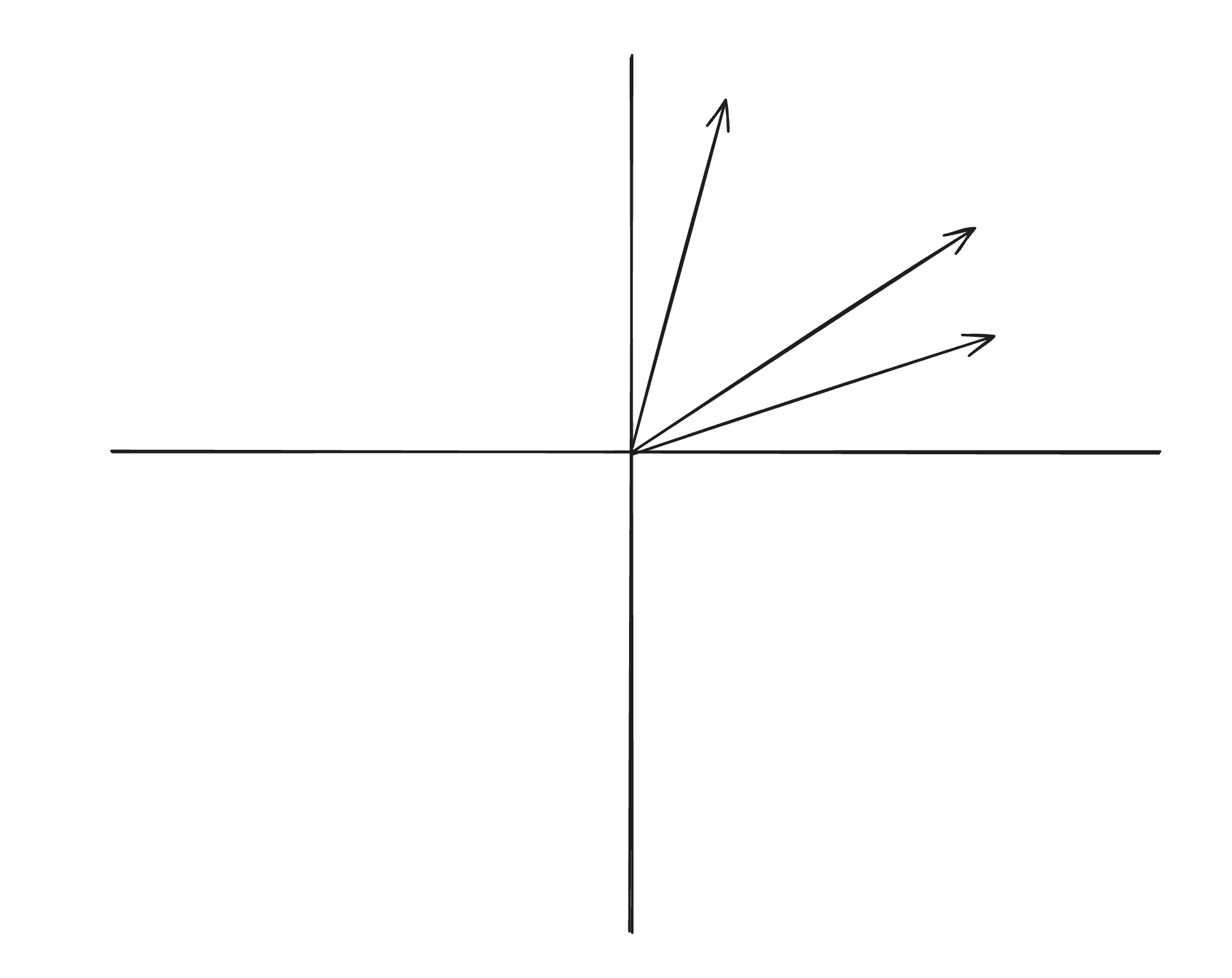
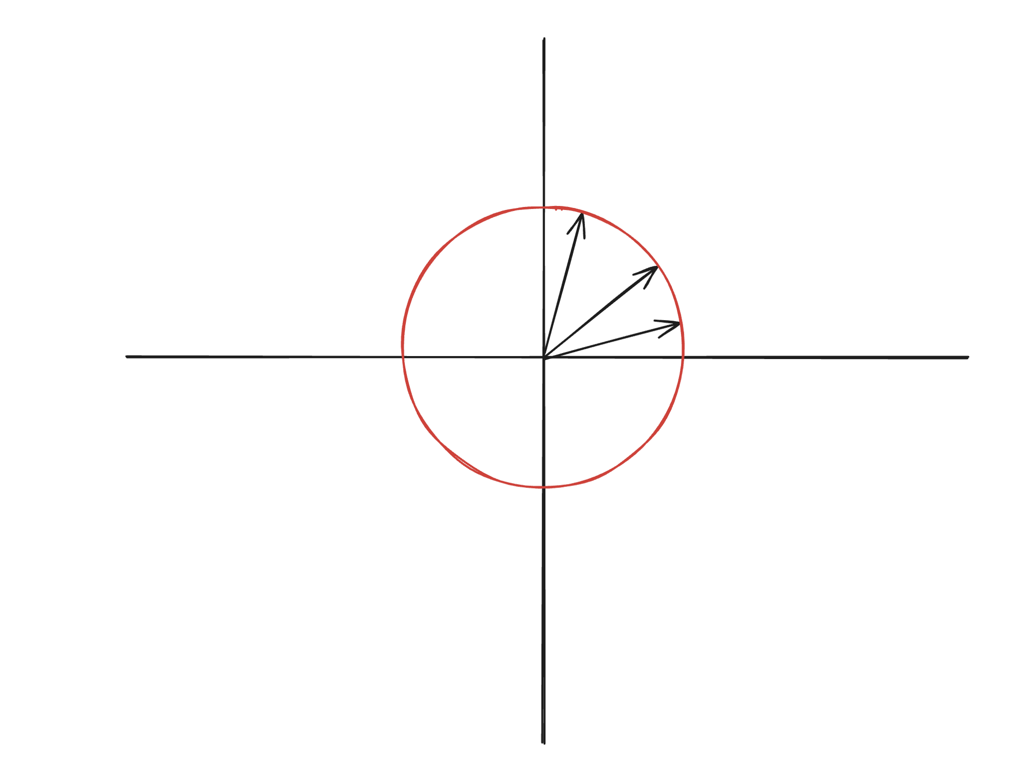
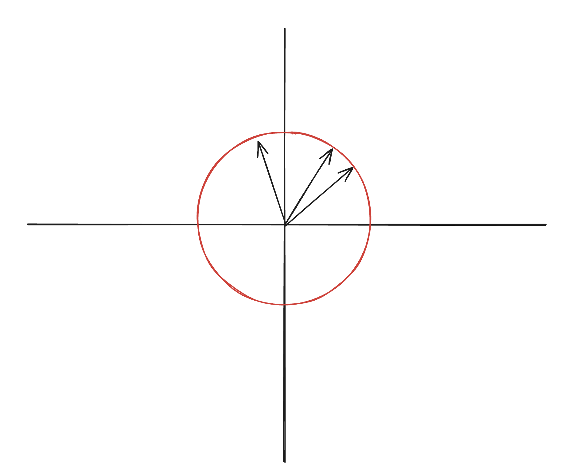
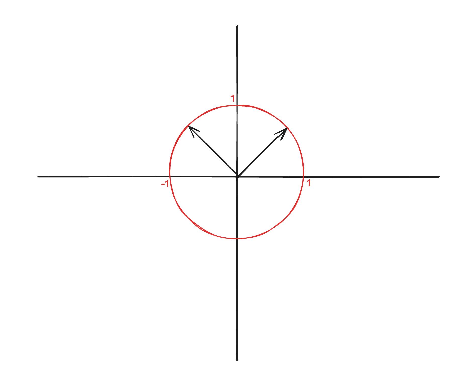
RaBitQ is a smart binary Quantisation method that leverages the property of high-dimensional space. The input vectors are normalised, and then a random rotation is applied.

1. Normalisation: all input vectors to unit length (i.e., project them onto the unit hypersphere).
2. Random Rotation: A random orthogonal transformation is applied to all input vectors.
3. Quantisation: After the transformation, each vector's coordinates are replaced with

or

Why does it need to be randomly rotated?

If we would just do the quantisation on the normalised vectors, then that construction may favour some certain vectors and perform poorly for others. For example, for the data vector:

it's quantised data vector (which corresponds to the vector closest from the original data vector) is: 

and it's squared distance to the quantised data vector is 0. In contrast, for the vector:

it's quantised data vector is also:

and it's squared distance to the quantised data vector equals to:

To deal with this issue, RaBitQ injects some randomness into the encoding, which drastically decreases the probability of such cases.

Why does this bit-quantisation work?

At first glance, reducing each dimension of a vector to a single bit may seem too aggressive, but in high-dimensional space, our intuitions often fail us. In essence, it preserves the vector sufficiently, it is enough to preserve the coordinate’s sign. The following math is leaving out some technical steps, and should not be considered as a direct proof, but it should give an idea why is this possible.

When you pick a random vector with 1000 dimensions

with standard normal coordinates, two facts combined make it's normalised first coordinate extremely tightly clustered around zero.

We can say the following abut the sum of the coordinates' squares:

It is by definition following Chi-square distribution

From this, we know that the random variable of the sum of squares has a k mean and a 2k variance. We can calculate that the probability of that the length of the vector differs from the square root of k more than let’s say 5 is basically zero.

The probability of that two cases can be computed since we know the of the sum of squares' distribution and it’s parameters:

which is astronomically small. Because of this, the coordinates' standard deviation can be estimated to be very small, around 0.03:

So we can conclude that an individual coordinate is most probably very small, because it has a mean of 0, and a very low standard deviation. That’s why storing only the sign of the given coordinate can be sufficient.
RaBitQ focuses on encoding angular information rather than exact spatial coordinates.

The IVFFLAT approach can be naturally extended to IVF_RABITQ, where we perform the clustering first, then normalisation is done relative to the closest cluster centroid, improving local encoding accuracy. Then it proceeds to randomly rotate and then quantise the vectors in each cluster, as discussed above.

Steps

1. Perform K-means (classical/spherical) clustering
2. Normalise all input vectors to unit length relative to it’s cluster centroid
   ( i.e., project them onto the unit hypersphere centered around the cluster centroid).
3. Random Rotation: A random orthogonal rotation is applied (which is different per each cluster)
   to all input vectors.
4. Quantise the vector, each vector's coordinates are replaced with     

or

according to their sign.

In query time, we look for the nprobe amount of nearest cluster centroids, put in the query vector and do the normalisation + rotation for each different cluster and we look for the closest quantised vectors. Note that the query vector does not get quantised.

Parameters

This index type aims to combine the fast query times thanks to quantisation, while retaining very high recall, and since it is an extension of IVFFLAT, also achieving fast index build times. 

Pros:

• Very fast index build times 
• Not sensitive to record deletion
• Fast query speeds thanks to the bit quantisation

Cons:

• Large amount of new entries require rebuilding of the index
• Not as widespread, few implementations

Conclusion

The most important is to be cautious about which index type and implementation suits our use case the best. In most cases HNSW will still be the best option rightfully so, but in other cases, where frequent index rebuilds are required, especially at large scale, IVFFLAT based approaches might end up being a better option.